Download Fibonacci Heap - Advanced Data Structures and Algorithms - Solved Exam and more Exams Data Structures and Algorithms in PDF only on Docsity!
Be neat and concise, but complete.
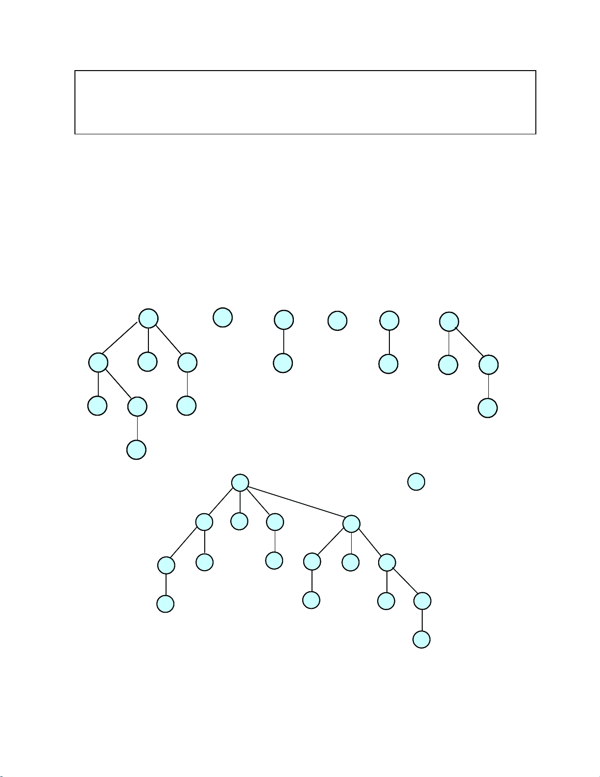
- (5 points) The figure below shows a single Fibonacci heap. The numbers next to the nodes
are the key values. The ranks are not shown. Show how the heap structure changes following a deletemin operation. Perform the linking steps from left to right – that is always combine the leftmost pair of trees that are “eligible” to be combined.
CS 542 – Advanced Data Structures and Algorithms
- Jonathan Turner 11/1/ Exam 2 Solutions - d 2 e^5 k - a 7 q - l - i - f 10 g - h - p
- o 6 b - n - m - r - j - c - d 2 ee^55 kk - a - dd - aa 77 q - l - qq - ll - i - f - ii - ff 1010 g - h - gg - hh
- o
- oo 66 b - n - bb - nn - m - r - mm - rr - j - c - jj - cc - k - e - q 6 a - l - i - f 10 g - h - p - o 6 b - n - m - j 7 r - c - kk - ee - q 6 aa - l - qq - ll - i - f - ii - ff 1010 g - h - gg - hh - p - o - pp - oo 66 b - n - bb - nn - m - r - mm - j 7 rr - c - jj - cc
- (10 points) Consider the graph shown below. Suppose we apply the general scanning and labeling method for shortest paths to this graph.
If the vertices are scanned in topological order, what is the total number of times that a vertex is scanned?
Each vertex is scanned once, so the total is 10.
Suppose the vertices are scanned in the most inefficient possible order. How many times are vertices scanned in this case? Explain.
The worst-case order is d, a, f, b, h, c, j, i, j, g, h, c, j, i, j, e, f, b, h, c, j, i, j, g, h, c, j, i, j. So, the total number of times vertices are scanned is 29.
Generalize the example to show that the scanning and labeling method can take Ω(2 n ) time in the worst-case.
Let the four node component at right (containing c, h, i and j) be called G 1. For k>1, we can form Gk by adding the component shown below “in front” of Gk–1. So for example, the graph above is G 3 , using these definitions. If n (^) k is the number of scanning steps in the worst-case scanning order for G (^) k , then
n k =3+2n k–1. This is Ω (2 k^ )= Ω (2 n).
4
d e
a
f 4 0
(^4 )
g
b
h 2 0
(^2 )
i
c
j
j
1 0
4 1
d e
a
f 4 0
(^4 )
g
b
h 2 0
(^2 )
i
c
j 1 0
1
2 k–^12 k–^1
2 k–^1
2 k–^12 k–^1
2 k–^1
- (15 points) Let G be a directed graph with each edge ( u , v ) having a non-negative capacity , cap ( u , v ). The bottleneck capacity of a path in G is the minimum capacity of one of its edges and a best bottleneck capacity path is one with the largest bottleneck capacity. A best bottleneck path tree is a spanning tree of G whose paths are best bottleneck paths.
Let T be a spanning tree of G with root s and let bcap ( u ) be the bottleneck capacity of the path from s to u in T. Show that if T is a best bottleneck path tree, then bcap ( v )≥min{ bcap ( u ), cap ( u , v )}, for all edges ( u , v ) in G.
If bcap ( v )<min{ bcap ( u ), cap ( u , v )} for some edge ( u,v ) then there is a path to v with a larger bottleneck capacity than the tree path, implying that T is not a best bottleneck path tree. Therefore, if T is a best bottleneck path tree then bcap ( v )≥ min{ bcap ( u ), cap ( u , v )}, for all edges ( u , v ) in G.
Show that if there is a non-tree path p from s to some vertex x , that has bottleneck capacity larger than bcap ( x ), then there must be some edge ( u , v ) for which bcap ( v )<min{ bcap ( u ), cap ( u , v )}.
Assume that p is a shortest path satisfying the condition and that path p has k edges. If k=1, p consists of the single edge (s,x) and has bottleneck capacity equal to cap(s,x)=min{bcap(s),cap(s,x)}, and since p is assumed to have larger bottleneck capacity than the tree path to x, it follows that bcap(x)<min{bcap(s),cap(s,x)}.
If k>1, let (w,x) be the last edge on p and note that since p is the shortest non-tree path with larger bottleneck capacity than the corresponding tree path, the tree path from s to w is a best bottleneck path. Consequently, the bottleneck capacity of p is at most min{bcap(w),cap(w,x)}. Since p has larger bottleneck capacity than the tree path to x, this means that bcap(x)<min{bcap(w),cap(w,x)}.
- (10 points) Consider an execution of the capacity scaling version of the augmenting path algorithm for maximum flows. Suppose that we’re at the start of a scaling phase, in which the scaling parameter is equal to 100, and that X is the set of all vertices that can be reached from the source vertex s , by paths with capacity of at least 200. Let X ′ be the set containing all other vertices.
Give an upper bound on the residual capacity of an edge with one endpoint in X and the other in X ′. Justify your answer.
The residual capacity of such an edge must be less than 200, since otherwise there would be a path with residual capacity 200 from s to the endpoint in X ′.
Suppose there are 40 edges that cross the cut ( X , X ′) that have residual capacity of at least 100 (from the endpoint in X to the endpoint in X ′). Give an upper bound on the number of augmenting paths that can be found before the end of this scaling phase. Justify your answer.
The number of augmenting paths is at most 79, since each path increases the flow crossing the cut by at least 100 and the edges have a residual capacity less than 200.
Suppose that in the original graph, all edge capacities are multiples of 25 and that the largest edge capacity is 400. Give an upper bound on the number of scaling phases in which at least one augmenting path is found. Justify your answer.
If we start with a scaling parameter of 400, the subsequent phases have scaling parameters of 200, 100, 50 and 25. Once we go past this, no further augmenting paths can be found, so there are at most 5 phases in which an augmenting path is found. The reason for this is that since the edge capacities are multiples of 25, the residual capacities will always be multiples of 25. This means that at the end of the phase with scaling parameter 25, there can be no augmenting path with a residual capacity less than 25, so subsequent scaling phases will not find a path.
- (10 points) The figure below shows an intermediate state in the execution of Dinic’s algorithm with dynamic trees. In the picture of the flograph, the adjacency lists are indicated by the arcs connecting the edges at each vertex, and the solid circles indicate the position of the nextedge pointers in the adjacency lists. So for example, nextedge ( c )=( b , c ) and nextedge ( g )=( g , i ) .The dynamic trees data structure is shown at right.
What is the flow on edge ( e , h )? 7
What is the residual capacity of edge ( f , t )? 6
Show the state of the dynamic trees data structure at the point the next search for an augmenting path reaches the sink. Be sure to show all the node costs.
g 2
s (^2)
d 4 c^3 b^4
e
f 6 i (^5) h (^1)
t H
gg 22
ss (^22)
dd 44 cc^33 bb^44
ee 22
ff 66 ii (^55) hh (^11)
tt HH
g H
s 2
c 3 b^4
d 4
e 2
f H
i
capacity, f low
c
d g
b e
t
f
i
h
h
h
h
1 h^1
t H
nextedge level
gg HH
ss 22
cc 33 bb^44
dd
ee 22
ff HH
ii
capacity, f low
c
d g
b e
t
f
i
h
1 hh^11
tt HH
nextedge level
Show the changes to the flow values in the flograph data structure after flow is added to the augmenting path found by this search. You may just mark the changes on the diagram above.
The revised version is shown below.
capacity, f low
s c
d g
b e
t
4,
6,
4, 1, 7,
2,
3,
8,
3,0 6,0 4,
3,
f
i
h
4,
5,
3,
8,
9,
2,0 8,
7,1 4
2
(^12)
1
0 3
3
3
1
capacity, f low
s c
d g
b e
t
4,
6,
4, 1, 7,
2,
3,
8,
3,0 6,0 4,
3,
f
i
h
4,
5,
3,
8,
9,
2,0 8,
7,1 4
2
(^12)
1
0 3
3
3
1